Mapping Visibility: Applying Zone of Theoretical Visibility Analysis to St Paul’s Cathedral
While researching spatial planning methodologies used in the renewable energy sector, I came across Zone of Theoretical Visibility (ZTV) analysis — a technique I hadn’t encountered in my coursework but which is fundamental to how wind farm applications are assessed in the UK planning system. Intrigued by the methodology, I decided to work through it myself before applying it to a more complex context.
What is a ZTV?
A ZTV is a map showing all locations from which a structure could theoretically be seen, based purely on terrain and elevation data. The word “theoretical” is important — it assumes no vegetation, no intervening buildings, and a clear atmosphere. In practice it represents a worst-case visibility envelope, which is exactly what planning authorities need when assessing the visual impact of a proposed development.
In the context of wind farm planning, ZTVs are produced to identify sensitive receptors — residential properties, roads, National Scenic Areas, and heritage sites — that fall within the theoretical visibility zone of proposed turbines. Cumulative ZTVs layer multiple proposed or consented sites to assess combined visual impact, which is increasingly significant in Scotland where offshore and onshore wind development is dense.
Why St Paul’s Cathedral?
I chose St Paul’s Cathedral as my case study for reasons that go beyond its recognisability. At 111m to the cross, it sits considerably lower than many of the towers surrounding it in the City of London — yet it benefits from some of the most legally robust visibility protections of any structure in the UK. The London View Management Framework (LVMF) designates a series of protected viewing corridors from locations across London — Parliament Hill, Kenwood, Primrose Hill and others — within which development height is strictly controlled to preserve sightlines to the Cathedral. This makes it an ideal test case: unlike a tall building where you are simply mapping what can be seen, here there is a statutory framework to cross-reference against the output.
A standard bare-earth Digital Terrain Model would produce an unrealistically open viewshed in this context, so I used a Digital Surface Model (DSM) incorporating building heights to ensure surrounding structures correctly occlude lines of sight.
Methodology
The analysis was conducted in QGIS 3.44 using a LiDAR-derived DSM, resampled to 5m resolution for processing efficiency. Processing steps were as follows:
Data preparation — The DSM was clipped to a defined area of interest centred on the City of London. All layers were confirmed in EPSG:27700 (British National Grid) to ensure metric accuracy throughout. Prior to analysis, scattered NoData pixels identified within the DSM were interpolated using the Fill NoData tool to prevent erroneous occlusion along sightlines.
Observer point — A polygon was placed at the St Paul’s dome apex. Because the DSM already encodes the Cathedral’s height as an absolute elevation value in metres ASL, the observer height was set to 0m — adding the structure height on top would have double-counted the ground elevation and produced an inflated result. This distinction between relative and absolute height handling is critical when working with surface models rather than terrain models.
Viewshed calculation — The Viewshed tool was run with a target height of 1.6m and an analysis radius of 20,000m. The binary output assigns a value of 1 to all cells with a theoretical line of sight to the observer point, and 0 to occluded areas.
Result
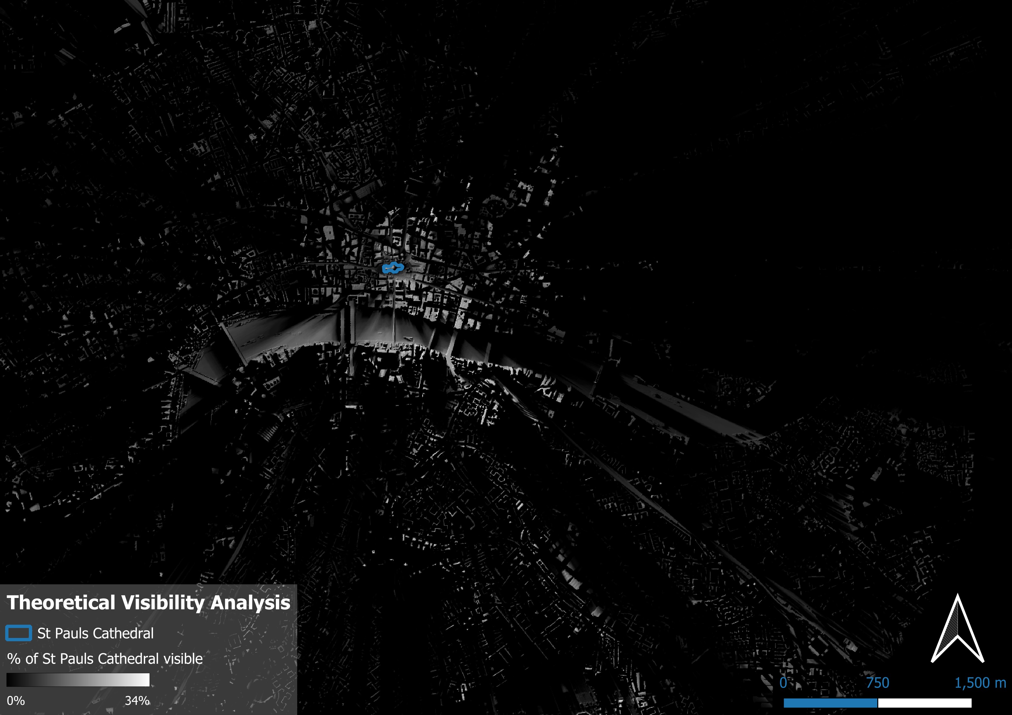
The output shows a visibility pattern consistent with the protected corridors designated under the LVMF. Sightlines extending northwest toward Parliament Hill, Kenwood and Primrose Hill — all statutory protected viewpoints — appear in the visible area of the output, broadly corroborating the planning framework’s basis in actual topography and urban form. The dense building fabric of the City itself creates significant occlusion at short range, while the Thames corridor and lower-lying areas to the east and southeast show greater theoretical visibility.
This cross-referencing of a GIS output against a statutory planning framework is precisely how ZTV analysis functions in practice — the map is not the end product but a tool for interrogating real planning constraints.
Relevance to Offshore Wind Planning
This exercise maps directly onto how ZTV analysis functions in a marine spatial planning context — the focus of my dissertation on spatial use conflicts in the Moray Firth. Offshore turbines present a different challenge: the absence of intervening structures over open water means visibility ranges are far greater, and the relevant receptors extend to coastal communities, shipping lanes, and designated landscapes. Understanding the mechanics of ZTV production — particularly the DSM versus DTM distinction and the implications for observer height — is a prerequisite for interpreting or producing these outputs in a professional context.
The technique is also directly relevant to cumulative impact assessment, where the interaction between multiple wind farm ZTVs must be mapped and communicated clearly to planning authorities and the public. This is an area I am keen to develop further.
Reflections
Working through this from scratch surfaced a number of methodological decisions that are easy to overlook when using a tool procedurally: the choice of surface model, the handling of NoData values, observer height in absolute versus relative terms, analysis radius, and the trade-off between raster resolution and processing time. At 5m resolution over a 20km radius the analysis took approximately 50 minutes — a useful reminder that in a professional context these decisions have real implications for project timelines, not just output quality.
The outputs for major renewable energy applications in Scotland may be tested at Public Inquiry, making methodological rigour not just academically important but professionally necessary.
Tools used: QGIS 3.44, Viewshed, Fill NoData, LiDAR DSM (resampled to 5m resolution)
All analysis conducted in EPSG:27700 (British National Grid)